Implementing SVM Classifier
If you are currently doing CS231n first assignment, Please be advised that article contains code implementation and now is the right time to close the tab.
Table of Contents:
- Loading the CIFAR10 dataset
- Pre-processing the data
- SVM Classifier Implementation
- Stochastic Gradient Descent
- Hyperparameter Tuning
- Visualizing Results
In my previous post, we have discussed about the disadvantages of K-NN classifier and how linear classification can help solve some of the problems. In this post, we are going to implement a multi-class linear support vector machine classifier.
Loading the CIFAR10 dataset
First things first, we need to load the data. Similar to our previous k-nn implementation, we are going to use CIFAR-10 dataset. CIFAR10 dataset contains 60,000 labeled images. These 60, 000 images are divided into 10 categories with each category containing 6000 images. Each image is of 32X32 resolution with each pixel containing 3 color bits. If you are following CS231n assignment this is already taken care for you.
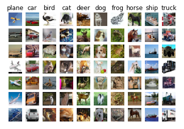 Figure 1: Samples of the CIFAR-10 Dataset
Pre-processing the data
Divide
We need to divide our dataset for training, testing, validation subsets. We also need a small dev subset from our training set for rough estimates of time consuming calculations.
Reshape
For computational efficiency, we need to reshape our images into single 3072 pixel array from existing 32X32X3 multi-dimensional array.
Following are sizes of our datasets
Training data shape:  (49000, 3072)
Validation data shape:  (1000, 3072)
Test data shape:  (1000, 3072)
dev data shape:  (500, 3072)
Substract Mean Image
Further to improve, we can substract mean pixel value of all images from each image. Mean Image that we substract looks like below
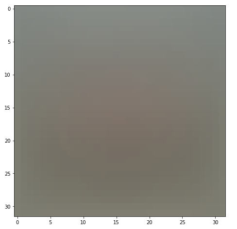
Figure 2: Mean Image of CIFAR-10 dataset
Append Bias Dimension
Remember our bias trick from Linear Classification post. We can have Bias dimension in our image data itself than separate entry which saves one additional calculation step.
Post this operation our dataset sizes looks like below
(49000, 3073) (1000, 3073) (1000, 3073) (500, 3073)All the logic required for Divide, Reshape, Substracting mean image and appending bias dimension are already taken care in the assignment notebook.
SVM Classifier Implementation
SVM Loss
SVM Loss is set up in such a way that correct class scores are higher than incorrect class scores by some fixed margin say . The loss function is defined as follows
Where represents predicted score of incorrect class and represents predicted score of correct class.
Regularization Loss
There is one problem with above way of calculating the loss. The problem is that there might be many weights for which the classifier can predict correctly. Classifier only cares about having some delta margin between true class and incorrect class, if we find another set of weights for which the margin is delta + k, even then we would get the same accuracy. The choice we are making here is to have minimum possible values of W, for which we need to introduce some penalty on over all loss function that grows as the value for W increases. This is done using L2 norm, which discourages large weights by adding elementwise quadratic penalty of all the parameters. Thus loss becomes
Regularization loss is weighted by , a hyperparameter that is usually determined by cross-validation.
Naive Loss Implementation
In naive loss implementation, we aren’t restricted by performance efficiency and have the freedom to understand the way loss is calculated and implement algorithm. We know that we have to add up losses of all class scores except the correct one if the score of it is greater than true class score by a margin. Best value for margin a.k.a is given as 1, you can read Course Notes for why.
Naive Loss Implementation
def svm_loss_naive(W, X, y, reg):
    """
    Structured SVM loss function, naive implementation (with loops).

    Inputs have dimension D, there are C classes, and we operate on minibatches
    of N examples.

    Inputs:
    - W: A numpy array of shape (D, C) containing weights.
    - X: A numpy array of shape (N, D) containing a minibatch of data.
    - y: A numpy array of shape (N,) containing training labels; y[i] = c means
      that X[i] has label c, where 0 <= c < C.
    - reg: (float) regularization strength

    Returns a tuple of:
    - loss as single float
    - gradient with respect to weights W; an array of same shape as W
    """
    # dW will be an array of shape (3073, 10) same as W
    dW = np.zeros(W.shape)  # initialize the gradient as zero

    # compute the loss and the gradient
    num_classes = W.shape[1]
    num_train = X.shape[0]
    loss = 0.0
    for i in range(num_train):
        # X is of shape (500, 3073), W is of shape (3073, 10)
        # Get the scores using Dot Product
        scores = X[i].dot(W)
        # Correct Class Scores can be found using Y[i] as index
        correct_class_score = scores[y[i]]
        for j in range(num_classes):
            #if correct closs skip the loss calculation for that class
            if j == y[i]:
                continue
            # find the margin
            margin = scores[j] - correct_class_score + 1  # note delta = 1
            if margin > 0:
                loss += margin
                # SVM Loss function is Sum(Max(0, W[j].T.dot(X[i]) - W[y[i]].T.dot(X[i]) + delta))
                # Since there is max function, derivative applicable only if Sum > 0
                # Partial derivative w.r.t W[y[i]] is substraction from dW
                # Partial derivative w.r.t W[j] is addition to dW
                # Gradient w.r.t W is -X[i] for true class
                dW[:, y[i]] -= X[i]
                # Gradient w.r.t X[i] for incorrect class
                dW[:, j] += X[i]

    # Right now the loss is a sum over all training examples, but we want it
    # to be an average instead so we divide by num_train.
    loss /= num_train
    # Divide all over training examples
    dW /= num_train

    # Add regularization to the loss.
    loss += reg * np.sum(W * W)

    # Add regularization
    dW += reg * W

    #############################################################################
    # TODO:                                                                     #
    # Compute the gradient of the loss function and store it dW.                #
    # Rather that first computing the loss and then computing the derivative,   #
    # it may be simpler to compute the derivative at the same time that the     #
    # loss is being computed. As a result you may need to modify some of the    #
    # code above to compute the gradient.                                       #
    #############################################################################

    return loss, dW
Vectorized Loss Implementation
SVM loss through vectorized implementation was pretty straight forward but gradient calculation, you might need to think for a while. Notes in the code.
def svm_loss_vectorized(W, X, y, reg):
    """
    Structured SVM loss function, vectorized implementation.

    Inputs and outputs are the same as svm_loss_naive.
    """
    loss = 0.0
    num_train = X.shape[0]
    dW = np.zeros(W.shape)  # initialize the gradient as zero
    delta = 1

    #############################################################################
    # TODO:                                                                     #
    # Implement a vectorized version of the structured SVM loss, storing the    #
    # result in loss.                                                           #
    #############################################################################
    # Scores will be of shape 500X10
    scores = np.dot(X, W)
    # Correct Class Scores after adding new axis will be of shape 500X1
    correct_class_scores = scores[np.arange(num_train), y][:, np.newaxis]
    # Substracting Correct Class Scores through Broadcasting
    # Keeping correct class loss in max function for now
    margin = np.maximum(0, scores - correct_class_scores + delta)
    # Making correct class loss to 0
    margin[np.arange(num_train), y] = 0
    # toClipboardForExcel(margin)

    # Summing Up Over All Loss
    loss = np.sum(margin)

    loss /= num_train

    # Adding Regularization Loss
    loss += 0.5 * reg * np.sum(W * W)
    #############################################################################
    #                             END OF YOUR CODE                              #
    #############################################################################

    #############################################################################
    # TODO:                                                                     #
    # Implement a vectorized version of the gradient for the structured SVM     #
    # loss, storing the result in dW.                                           #
    #                                                                           #
    # Hint: Instead of computing the gradient from scratch, it may be easier    #
    # to reuse some of the intermediate values that you used to compute the     #
    # loss.                                                                     #
    #############################################################################
    # This mask can flag the examples in which their margin is greater than 0
    count = np.zeros(margin.shape)
    #Set the value as 1 for those that are predicted incorrectly
    count[margin > 0] = 1

    # Sum all incorrect predictions for a particular image
    no_of_incorrect_predictions = np.sum(count, axis=1)
    # For all correct image score substract number of incorrect predictions
    count[np.arange(num_train), y] = -no_of_incorrect_predictions
    # Dot product for derivative
    dW = X.T.dot(count)

    # Divide the gradient all over the number of training examples
    dW /= num_train

    # Regularize
    dW += reg * W
    #############################################################################
    #                             END OF YOUR CODE                              #
    #############################################################################

    return loss, dW
Stochastic Gradient Descent
Now that we have calculated the loss and Gradient Descent, we can proceed further to reduce the loss. Stochastic Gradient Descent also known as incremental gradient descent is the process through which we iteratively optimize the input function through differentiation.
Since we have already calculated the gradient w.r.t W, all we have to do is update our parameters towards the direction of our gradient. I have updated the weights in the train method of the classifier.
self.W -= grad * learning_rateAfter 1500 iterations of training, following are the loss values.
iteration 0 / 1500: loss 404.773550
iteration 100 / 1500: loss 240.415640
iteration 200 / 1500: loss 147.031670
iteration 300 / 1500: loss 89.381552
iteration 400 / 1500: loss 56.038321
iteration 500 / 1500: loss 35.140617
iteration 600 / 1500: loss 23.027359
iteration 700 / 1500: loss 16.490472
iteration 800 / 1500: loss 11.874656
iteration 900 / 1500: loss 9.655397
iteration 1000 / 1500: loss 7.084481
iteration 1100 / 1500: loss 6.302023
iteration 1200 / 1500: loss 6.409429
iteration 1300 / 1500: loss 5.617606
iteration 1400 / 1500: loss 5.532514
That took 7.569127s
If we plot the loss over iterations, Graph would look like below.
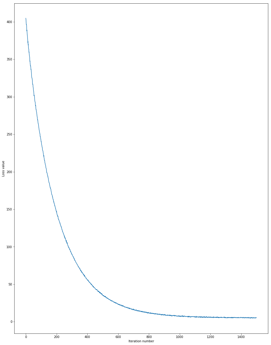
Figure 3: Loss over Iterations
With the current weight parameters if we try to predict the labels on training and validation set, you would see an accuracy around 40%.
training accuracy: 0.383571
validation accuracy: 0.393000
Hyperparameter Tuning
Right set of Learning Rate and Regularization Strengths are important for the loss function to converge. Since, there is no right number for us to use right away. The approach we are using is brute force, kind of testing all the possible values that we think should be good. We will be training batch of 200 images with 1500 iterations for every possible learning rate and regularization strength and store the best accurate model hyper parameters.
Following is the code that’s implemented for storing accurate model
for lr in learning_rates:
    for reg in regularization_strengths:
        svm = LinearSVM()
        svm.train(X_train, y_train, learning_rate=lr, reg=reg, num_iters=1500, batch_size=200)
        y_train_pred = svm.predict(X_train)
        y_val_pred = svm.predict(X_val)
        training_accuracy = np.mean(y_train == y_train_pred)
        validation_accuracy = np.mean(y_val == y_val_pred)
        results[(lr, reg)] = (training_accuracy, validation_accuracy)
        if validation_accuracy > best_val:
            best_val = validation_accuracy
            best_svm = svm
I have tried out many different learning rates and regularization strengths before arriving at 1e-7, 2e4 for learning rate and regularization strength with help of web search.
learning_rates = [1e-8, 1e-7, 2e-7]
regularization_strengths = [1e4, 2e4, 3e4, 4e4, 5e4, 6e4, 7e4, 8e4, 1e5]
For the above parameters, following is the log of accuracy
lr 1.000000e-08 reg 1.000000e+04 train accuracy: 0.223367 val accuracy: 0.240000
lr 1.000000e-08 reg 2.000000e+04 train accuracy: 0.234755 val accuracy: 0.241000
lr 1.000000e-08 reg 3.000000e+04 train accuracy: 0.240898 val accuracy: 0.263000
lr 1.000000e-08 reg 4.000000e+04 train accuracy: 0.249143 val accuracy: 0.255000
lr 1.000000e-08 reg 5.000000e+04 train accuracy: 0.247531 val accuracy: 0.279000
lr 1.000000e-08 reg 6.000000e+04 train accuracy: 0.267673 val accuracy: 0.279000
lr 1.000000e-08 reg 7.000000e+04 train accuracy: 0.269551 val accuracy: 0.284000
lr 1.000000e-08 reg 8.000000e+04 train accuracy: 0.281592 val accuracy: 0.285000
lr 1.000000e-08 reg 1.000000e+05 train accuracy: 0.297020 val accuracy: 0.295000
lr 1.000000e-07 reg 1.000000e+04 train accuracy: 0.376673 val accuracy: 0.361000
lr 1.000000e-07 reg 2.000000e+04 train accuracy: 0.386735 val accuracy: 0.395000
lr 1.000000e-07 reg 3.000000e+04 train accuracy: 0.373367 val accuracy: 0.378000
lr 1.000000e-07 reg 4.000000e+04 train accuracy: 0.369714 val accuracy: 0.398000
lr 1.000000e-07 reg 5.000000e+04 train accuracy: 0.369898 val accuracy: 0.362000
lr 1.000000e-07 reg 6.000000e+04 train accuracy: 0.362367 val accuracy: 0.375000
lr 1.000000e-07 reg 7.000000e+04 train accuracy: 0.360612 val accuracy: 0.366000
lr 1.000000e-07 reg 8.000000e+04 train accuracy: 0.360980 val accuracy: 0.372000
lr 1.000000e-07 reg 1.000000e+05 train accuracy: 0.354347 val accuracy: 0.365000
lr 2.000000e-07 reg 1.000000e+04 train accuracy: 0.382551 val accuracy: 0.400000
lr 2.000000e-07 reg 2.000000e+04 train accuracy: 0.386061 val accuracy: 0.401000
lr 2.000000e-07 reg 3.000000e+04 train accuracy: 0.375857 val accuracy: 0.377000
lr 2.000000e-07 reg 4.000000e+04 train accuracy: 0.365469 val accuracy: 0.370000
lr 2.000000e-07 reg 5.000000e+04 train accuracy: 0.354265 val accuracy: 0.369000
lr 2.000000e-07 reg 6.000000e+04 train accuracy: 0.351449 val accuracy: 0.372000
lr 2.000000e-07 reg 7.000000e+04 train accuracy: 0.347816 val accuracy: 0.369000
lr 2.000000e-07 reg 8.000000e+04 train accuracy: 0.342102 val accuracy: 0.351000
lr 2.000000e-07 reg 1.000000e+05 train accuracy: 0.346980 val accuracy: 0.375000
best validation accuracy achieved during cross-validation: 0.401000
Accuracy is between 24% to 40.1%.
Visualizing Results
Its always good to see the numbers plotted in a graph and on top of it we already have logic pre-filled in the assignment notebook for us to visualize accuracies for different hyperparameters, beat that.
Accuracy of Hyperparameters
The default color map is black and white, I felt that white was mixing into the background of the plot so changed the plot colors. They look like below
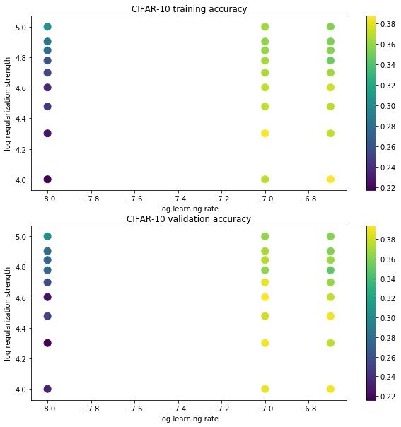
Figure 4: Accuracy and Hyperparamters
Weight Parameters
One of the analogy of weight parameters is to imagine weight parameters as a template for the class. If we print the the learned weight parameters as an image after compensating for the substracted mean image of input vector. We can clearly see patterns of the class. From each image of different class such as Front Facing Red Car, Front Facing Plane, Horse with two Heads, Green color frog through which we can derive some conclusions but gist of the story is that learned weights are nothing but a template of all the training images.
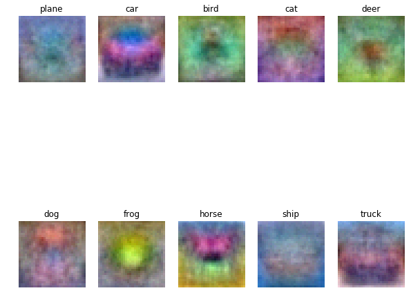
Figure 5: Learned Weight as Image
Final Thoughts
Although accuracy of 40% is not something we would want but this approach is indeed much better than remembering all the training images as in K-NN. Who would have thought that weights would end up as templates for the training images, definitely I didn’t until I saw the output. I was thinking of creating a template myself in photoshop by merging all the training images into one layer but again that would be challenging and require quite a bit of efforts as I would have to control each pixel’s opacity but not entire image opacity when I overlay images onto one layer. Eitherway, this is fun :).