Introduction to Linear Classification
In my previous post, I have covered implmentation of K-NN classifier, in this post we are going to discuss basics of Linear Classification
Linear Classification
In our previous post, we have used K-NN classifier to classify images into labels with an accuracy of around 27% on CIFAR-10 dataset. Fundamentally, we have three issues with K-NN in image classification
- Classification happened at run time, which meant comparing all training images
- Need to store entire training dataset for classification
- Finally, Accuracy
Let’s keep that in mind as we proceed to Linear Classification. In Linear Classification, we will assume that each image in the training set can form a linear vector in n-dimensional space as a decision boundary to classify the images. As we train with different images, we will adjust this linear vector. We should have those number of linear vectors as the number of labels for all the possible dimensions of the input data. So what we do ?.
Parametric Approach
Let’s do the math with easiest linear function. So let’s pick a line equation . Umm, x here is an image and y here is a label. So x must be a vector of image dimension and y must be the number of labels, right. Okay, so mx, c must be of same dimensions as y.
In case of CIFAR-10 dataset, we know label data shape is 10X1 and shape of one image image is 3072X1. Hence m has to be 10X3072 and c has to be of shape 10X1. So far, the explanation was in terms of traditional linear algebra but in machine learning terms will change. Slope will be Weight and C (Y-intercept) will be bias.
Now you may ask, what’s the advantage. What we are doing through this linear equation is that, we are trying to find appropriate weight and bias paramaters that appropriately fits training set and performs well on validation set. This will help reduce the enormous training set into weight and bias parameters and we will be able to classify unseen data through single matrix multiplication. Isn’t that awesome ?.
Now, the question is how do we choose this weight and bias parameters. Well, we know the true output that we want and based on that we have to adjust weight and bias parameters. But, how can we do that. Here comes the concept of score and loss functions. Score Function is the result of the linear classifier and the loss function(also referred as cost function) is the deviation of the linear classifier from true score. Our goal is to iteratively modify the parameters and find suitable parameters for which loss is minimum.
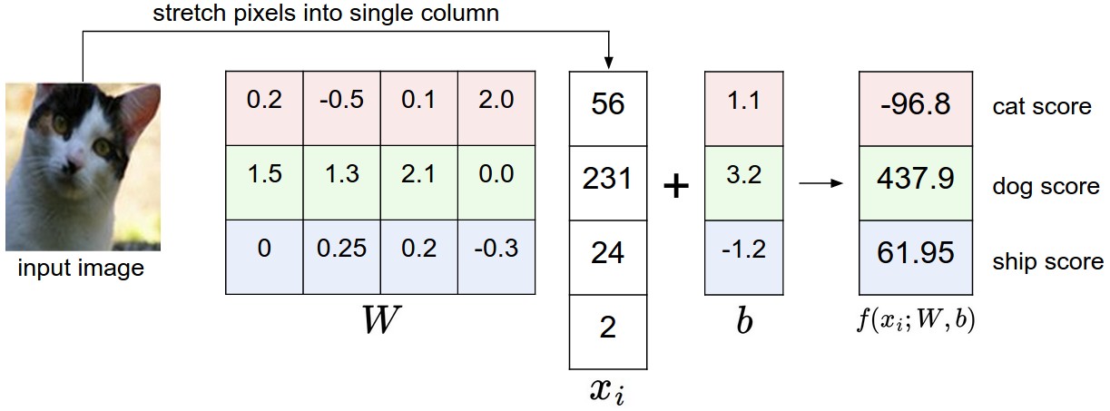 Figure 1: Parametric Approach Visualization. Source: CS231n Course, MIT
Bias Trick
In the above score function that we have, we are keeping tracking two different parameters in two different sets and actually we can combine them to simplify the score function. What we do is combine bias and together and represent both of them as . You may wonder how, all we need to do is move the bias values into Weight parameters and add one dimension to x with values as 1, so instead of 10X3072 weight, we will have 10X3073 and instead of 3072X1 x dimension we will have 3073X1.
Picking appropriate score function and loss function is critical in machine learning process. There are different algorithms and each have their own advantages and disadvantages. Since we are using linear regression algorithm as our score function, let’s talk about the loss function.
Loss Function
We can go in length discussing about what’s a loss function and what are different loss functions that are available that we can use but for now let’s pick one loss function and discuss about it.
Multiclass Support Vector Machine loss
Before we talk about Multiclass Support Vector Machine loss, let’s talk about Support Vector Machines in general. Support Vector Machines are supervised learning models used for classification and regression problems. They can be used for both linear and non-linear classification problems. There is one awesome video on Support Vector Machines by Professor Patrick Winston on MIT Open Courseware and is a must watch if you want to know about SVM.
Once you have gone through SVM, you will know that SVM expects the margin between correct and incorrect class to be as high as possible. Multiclass SVM loss for an ith example is given as
But there would be one problem in above scenario, there would be multiple weights for which there is minimum loss. To overcome that problem, regularization loss is introduced to offset the possibilities that we have for weights.
The full formula is
These formulas might seem daunting initially but when you apply you will realize that it is not so complicated after all. Having said that, understanding classifiers and loss functions is time consuming but you should spend every ounce of your energy to understand and learn how the models work. Hopefully, over a period of time we will get comfortable.
There are many different loss functions which deserve their own post. I suggest to take one at a time if you are beginner to ML.
Update:
2018-12-24: Added index